Faith, Decision Making and Probability III:
Bayes’ Theorem and the Anthropic Principle

But is it possible that probability brings certainty?
—Blaise Pascal, “Pensees,” 496

This is the third article in a series on faith, probability and decision making.  The first dealt with faith, some elementary rules of probability, and Pascal’s Wager.  The second focused on interpretations of probability.  In this post I’ll give some more lessions on probability rules (conditional probability, joint probability) and discuss Bayes’ Theorem, a method to update belief on the basis of new information.

Joint Probability, Conditional Probability

Let’s return to the example of different colored dice, one red die and one green die. Let’s suppose we put small weights behind the one dot face of the red die and the one dot face of the green die. To make the example concrete, let’s suppose the probabilities of 1 and 6 dots coming up on the dice are given as below:

• six dots, green die:  P( 6 | green) = 1/4  (= 1/6 + 1/12);  Event E1
• one dot, green die:  P( 1 | green) = 1/12 (= 1/6 – 1/12);   Event E2
• six dots, red die:      P( 6 | red)     = 1/4 (= 1/6 + 1/12);   Event E3
• one dot, red die:      P( 1 | red)      =  1/12  (= 1/6 – 1/12);  Event E4

Now a joint probability of two events is the probability of both of two events occurring, which I’ll denote by the simple “AND” (there’s a logical symbol for this, but why make things more complicated than necessary?)   Thus, (E1 and E3)  denotes the green die shows 6 dots and the red die shows 6 dots;  (E1 and E4) denotes the green die showing six dots and the red die showing one dot.   If the two events are independent, that is to say if what happens in one event doesn’t effect what happens in the other, then the probability of the joint event is simply the product of the probabilities for either.    So we can write

• P(E1 and E3) = 1/4 x 1/4 = 1/16;  6 dots green, 6 dots red, total 12 (1/6 x 1/6 = 1/36 if unweighted);
• P(E1 and E4) = 1/4 x 1/12 = 1/48;  6 dots green, 1 dot red, total 7;
• P(E2 and E3) = 1/12 x 1/4  =  1/48; 1 dot green, 6 dots red, total 7;
• P(E2 and E4)  = 1/12 x 1/12  = 1/144;  1 dot green, 1 dot red, total 2.

Now if we throw a large number of times, can we determine that the dice are loaded?  For a very large number of times, the probability of throwing a total of 2 would be 1/36 if the dice were fair and 1/144 if the dice were loaded; and similarly for throwing 12, the  probability would be 1/36 if the dice were fair, and 1/16 if the dice were loaded.  Clearly if, after a very large number of throws,  we came up with a ratio for a total of 12 close to  1/16, 2.5 times greater than 1/36, we might be suspicious that the dice were loaded.  If the number of throws were not so large, then it would be harder to tell.  Note that the observed probabilities for totals of 7 would only be slightly different from that if the dice were fair: 3/36 + 2/48  compared to 5/36, or 9/72 versus 10/72.

Bayes’ Theorem

The other strand of inductive probability treats the probabilities of theories as a property of our attitude towards them; such probabilities are then interpreted, roughly speaking, as measuring degrees of belief. This is called the subjectivist or personalist interpretation. The scientific methodology based on this idea is usually referred to as the methodology of Bayesianism because of the prominent role it assigns to a famous result of the probability calculus known as Bayes’s Theorem.
—C. Howson and P. Urbach, “Scientific Reasoning: the Bayesian Approach”

Let me just say what Bayes’ theorem and Bayesian analysis are all about.   Supposing, as in our example of the loaded dice, you know the probability of an event E (a total of 2 coming up) if the dice are loaded  (in our example, 1/48 compared to 1/36 for fair dice).   From the observed relative frequency of a total of 2 coming up, it is possible  to work backwards to figure out the probability that the dice are loaded.  Bayes’ Theorem will play a part in this, but one needs to invoke probability distribution laws also.

A well known example of Bayes’ Theorem application is the Monty Hall problem (see here and here for nice expositions of this.) It is particularly apt in that it shows how new information can modify probabilities.  I’ll give another example  drawn from medical tests.

Suppose there’s a rare disease, Quivers Antarctica (QA); only 0.2 % of the population have the disease QA, which is carried by penguins from the Antarctic.  Diagnostic tests for the disease QA are good: 99% sensitivity (99% of the people who have the disease test positive for it); 98% specificity (98% of the people who don’t have the disease test negative.   In a panoply of tests given to you for a job interview you find that you test positive for QA.

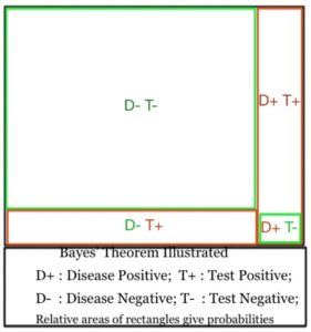Should you be worried?  Let’s look at the possibilities (and probabilities).  To save time writing I’ll use the shorthand notation given in the illustration to the right for positive, negative disease (D+, D-, respectively); positive, negative tests that say you have or don’t have the disease (T+, T-, respectively.)

So what’s the probability that you actually have the disease if you test positive?   It’s simply the ratio of people having the disease who test positive to the total number of people testing positive.  In the illustration it would be the ratio of the area D- T+ to the total area testing positive, area D-T+  plus area D+T+

Let’s tabulate this to make it clearer:

• P(D+) = 0.002 (incidence of disease)
• P(T+| D+) = 0.99 (sensitivity: probability of testing positive if disease present)
• P(T- | D-)  = 0.98 (specificity: probability of testing negative if disease absent)
• P(T+ | D-) = 1 – P(T- | D-) = 0.02 (probability of testing positive if disease absent)

Here are the numbers put into the formula for Bayes’ Theorem (Eq. 3, Note):

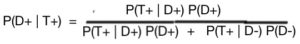
= P(T+| D-)/ P(T+)

= (0.99 x 0.002)/ [ (0.99 x 0.002) + (0.02 x 0.998) = 0.0902

To sum up: in both the classic Monty Hall problem and diagnostic test example, Bayes Theorem, working backward from new evidence to modify probabilities, supports the subjective interpretation of probability;  the use of Bayes’ theorem modifies belief. (But it has to be applied correctly.)  In the Monty Hall problem, the choice of door is changed to give an increased probability of winning;  in the diagnostic test example, the positive test gives only a 9% chance of having the disease rather than 99% when the possibility of incorrect test results is taken into account.

An Application to the Anthropic Principle

The Anthropic Principle is the notion that many physical laws, constants and situations are set up so that our universe can sustain carbon-based life.   The combination of these events, the so-called “anthropic coincidences,” is unlikely and tempts some to apply probability considerations.  One bad example of this is given here, where the author sets up a “Hashem equation,” a string of unlikely events, assigns a probability to each and gets a joint probability which is incredibly small.

I’ve written at length about this here and here, so I’ll just summarize those articles in this section.  The unlikely events and situations of the anthropic coincidences cover all of science: cosmology, particle physics, the laws of physics, geology, biology, chemistry.  Probabilities cannot be assigned to individual anthropic coincidences because they are interconnected in a framework of fundamental physical laws, laws that tell us about the the way the universe is, and are a consequence of how God created the universe.  

Nevertheless, one can use a form of Bayes’ Theorem, starting from Equation (2) in the Note, to show that knowledge of the anthropic coincidences can lead agnostics to belief in God, even though they won’t convince evangelical atheists (e.g. Richard Dawkins or Sean Carroll).  Quotes from two such believers are given below:

1. Fred Hoyle, who derisively termed the theory that the universe originated from a singularity, “The Big Bang,”  and who came from non-belief to faith: “A commonsense interpretation of the facts suggests that a super-intellect has monkeyed with physics, as well as chemistry and biology, and that there are no blind forces worth speaking about in nature.”
2. Anthony Flew, a British Philosopher, who announced his change from atheist to theist at the age of 81 with the quote “ ‘I’m thinking of a God very different from the God of the Christian and far and away from the God of Islam, because both are depicted as omnipotent Oriental despots, cosmic Saddam Husseins,’ he said. ‘It could be a person in the sense of a being that has intelligence and a purpose, I suppose.’ ” (as quoted by NBC News,)

And the anthropic coincidences may not lead to belief in the Christian God.  Grace is the toll for the road to Christ, not Reason.

NOTE: Derivation of Bayes’ Theorem

In order to derive Bayes’ Theorem we need to explore the relation of joint and conditional probabilities.   Here’s the basis, a fundamental rule relating conditional and joint probabilities:

P(E and B) = P(E | B)P(B).

If E and B are independent, then the probability of E doesn’t depend on whether B is true.   Then P(E | B) = P (E), i.e. the probability  of B is irrelevant. In this case P(E and B) = P(E) P(B).  An example would be the event, 4 dots on the red die, 2 dots on the green die; the probability would be 1/36 whether or not the dice were loaded: P(red 4 dots, green 2 dots | dice loaded) = P (red 4 dots, green 2 dots | dice fair) = P (red 4 dots, green 2 dots) = 1/36.   Now we can also write

P(E and B) = P(B | E) P(E)

where P(B | E) is the probability that belief B is true given event E happens. Combining the two relations for conditional and joint probability gives

P(E | B) P(B) = P(B | E) P(E),   (1)

or rearranging that,

(2)

that is to say, the probability that the belief B is true, given that the event E occurs, is equal to the probability that the event E occurs, given that the belief B is true, times the ratio of the probabilities of B and E.

Now, let’s suppose we have two mutually exclusive beliefs:  B and notB.  If B is true, notB isn’t, and vice versa. (For example:  B—the dice are fair;  notB—the dice are loaded.)  The P(B) + P(notB) = 1 (either one or the other of the two beliefs must be true).  Then we can write P(E)= P(E | B) P(B) + P(E | notB) P(notB).    The last equation above can then be rewritten as

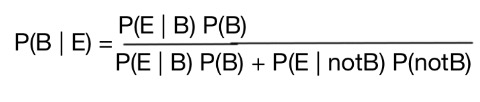
(3)

since P(E) is equal to the expression in the denominator;  this is the “traditional” form for Bayes’ Theorem. Gamblin Joe could use this expression to figure out how often he should use loaded dice (i.e set P(B)) so that the probability of snakeyes coming up would only give a 50/50 indication that the dice were loaded (i.e. that P(B | E) = 1/2).